If you do a simple image search for RNNs you will come across a myriad of images that all closely resemble this:
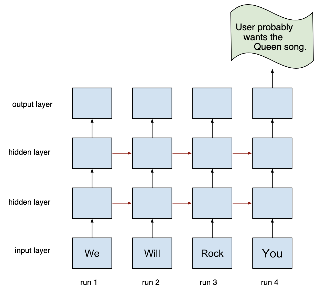
I think these diagrams are incredibly misleading because they don't convey the most important aspect of RNNs, which is that they are recurrent. One of the first things you see if you look up recursion is a picture of a serpent eating its own tail forming a cycle. Drawings that depict a linear flow can be completely misleading because there is no strong indication that recursion is taking place. These flattened diagrams show sequential time steps but it's not always clear that the RNN from one time step to the next is the same object. In some cases it's also not clear that moving from left to right means travelling through time and not different cells of a neural network.
from torch import nn


class SimpleRNN(nn.Module):
    def __init__(self, input_size, output_size, hidden_dim, n_layers):
        """
        Args:
            input_size (int): number of features of input data
                        full input data has sahpe (time, input_size)
            output_size (int): target shape to predict
            hidden_dim (int): number of 'features' in the hidden state
            n_layers (int): number of hidden layers, typically between 1 and 3
                            1+ would make a stacked RNN where the output of the
                            1st -> 2nd -> output

        """
        super(SimpleRNN, self).__init__()
        self.hidden_dim = hidden_dim
        # define the RNN
        self.rnn = nn.RNN(
            input_size,
            hidden_dim,
            n_layers,
            # ensures that 1st dimension is batch size
            batch_first=True)
        # fully connected layer input: output of RNN (hidden_dim) -> (output shape)
        self.fc = nn.Linear(hidden_dim, output_size)

    def forward(self, x, hidden):
        """
        Forward propagation.

        Args:
            x (tensor): input data tensor
                        shape: (batch_size, seq_length, input_size)
            hidden (tensor): initial hidden state for each element in the batch
                             shape: (n_layers * num_directions, batch_size, hidden_dim)
                             where num_directions is 2 if bidirectional, else 1
                             Defaults to zero if not provided.

        Returns:
            tensor: output from final fully connected layer
                    shape: (batch_size, seq_len, hidden_size)
                    tensor containing the output features (h_t)
            tensor: tensor containing hidden state @ t=seq_len
                    shape: (n_layers, batch_size, hidden_dim)

        """
        print("input data shape {}".format(x.shape))
        if hidden is not None:
            print("input hidden shape {}".format(hidden.shape))
        # get RNN outputs
        print("input -> RNN -> output, hidden state")
        r_out, hidden = self.rnn(x, hidden)
        print("RNN output {}".format(r_out))
        print("RNN h_n {}".format(hidden))
        # shape output to be (batch_size*seq_length, hidden_dim) for final layer
        r_out = r_out.view(-1, self.hidden_dim)
        print("final FC layer input shape {}".format(r_out.shape))
        # get final output
        output = self.fc(r_out)
        print("final output from FC layer shape {}".format(output.shape))
        return output, hidden
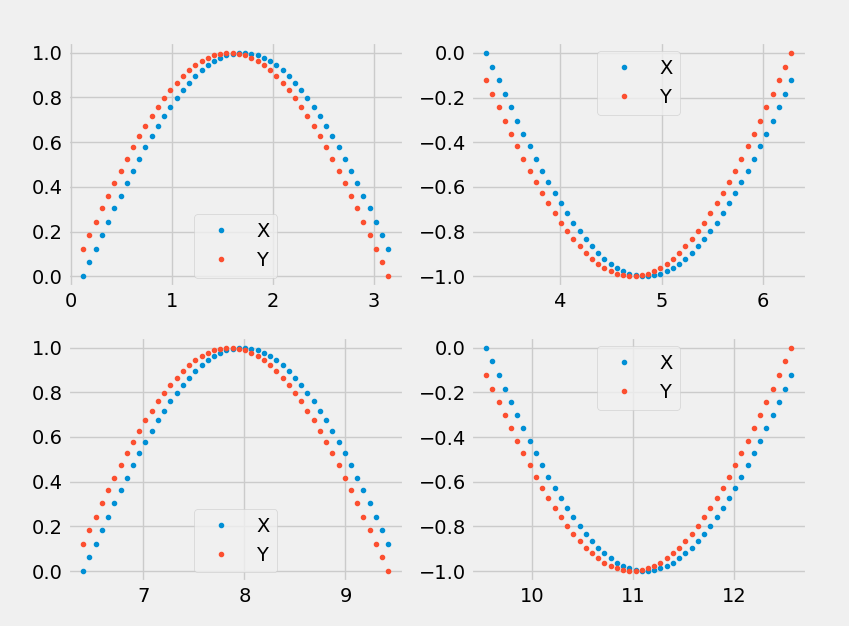
Let's make up some simple data. I'll use a sine curve and simply shift it for the target Y.
import numpy as np

def generate_training_data(seq_len, x_shift):
    """
    Generate some training data: a shifted sine curve.
    Produces

    Args:
        seq_len (int): the "vertical" dimension for 1 batch of data
        x_shift (int): translation of sine curve in x-axis

    Returns:
        array: x_dim to plot against
        tensor: input data
                shape: (1, seq_len, 1)
        tensor: target data
                shape: (seq_len, 1)

    """
    time_steps = np.linspace(x_shift * np.pi, (x_shift + 1) * np.pi, seq_len + 1)
    sine = np.sin(time_steps)
    x = sine[:-1, np.newaxis]  # all but the last piece of data
    y = sine[1:, np.newaxis]  # all but the first
    # create batch size dimension
    x_tensor = torch.Tensor(x).unsqueeze(0)
    y_tensor = torch.Tensor(y)
    return time_steps, x_tensor, y_tensor
Here's a sample of what our fake data looks like.
Now let's train the RNN on our made up data.
import matplotlib.pyplot as plt
import torch

# train the RNN
def train(rnn, criterion, optimizer, n_steps, seq_len=20, print_every=1):
    """
    Train the RNN.

    Args:
        rnn (nn model): instance of SimpleRNN
        criterion (loss):
        optimizer (optim):
        n_steps (int): 1 step = train with 1 batch of fake data
        seq_len (int): the "vertical" dimension of 1 batch of data
        print_every (int): how often to show loss

    """
    # initialize the hidden state
    hidden = None

    for step in range(n_steps):
        # make up training data for each step
        time_steps, x_tensor, y_tensor = generate_training_data(seq_len, step)

        # outputs from the rnn
        prediction, hidden = rnn(x_tensor, hidden)

        # memory: make new variable for hidden to detach it from its history
        # this way, we don't backpropagate through the entire history
        hidden = hidden.data

        # calculate the loss
        loss = criterion(prediction, y_tensor)
        # zero gradients
        optimizer.zero_grad()
        # perform backprop and update weights
        loss.backward()
        optimizer.step()

        # display loss and predictions
        if step % print_every == 0:
            print('Loss: ', loss.item())
            plt.plot(time_steps[1:], x_tensor.numpy().flatten(),
                     '.', label="input")  # true y
            plt.plot(time_steps[1:], prediction.data.numpy().flatten(),
                     '.', label="output")  # predictions
            plt.legend()
            plt.show()

    return rnn
Let's do a very small amount of training just to see that the model is working.
# decide on hyperparameters
input_size = 1  # 1 feature
output_size = 1  # 1 output
hidden_dim = 5  # let's keep this small for ease of inspection
n_layers = 1

# instantiate RNN
rnn = SimpleRNN(input_size, output_size, hidden_dim, n_layers)
print(rnn)
# simple MSE loss and Adam optimizer with a learning rate of 0.01
criterion = nn.MSELoss()
optimizer = torch.optim.Adam(rnn.parameters(), lr=0.01)

# train the rnn and monitor results
trained_rnn = train(rnn, criterion, optimizer,
                    seq_len=20, n_steps=40, print_every=10)
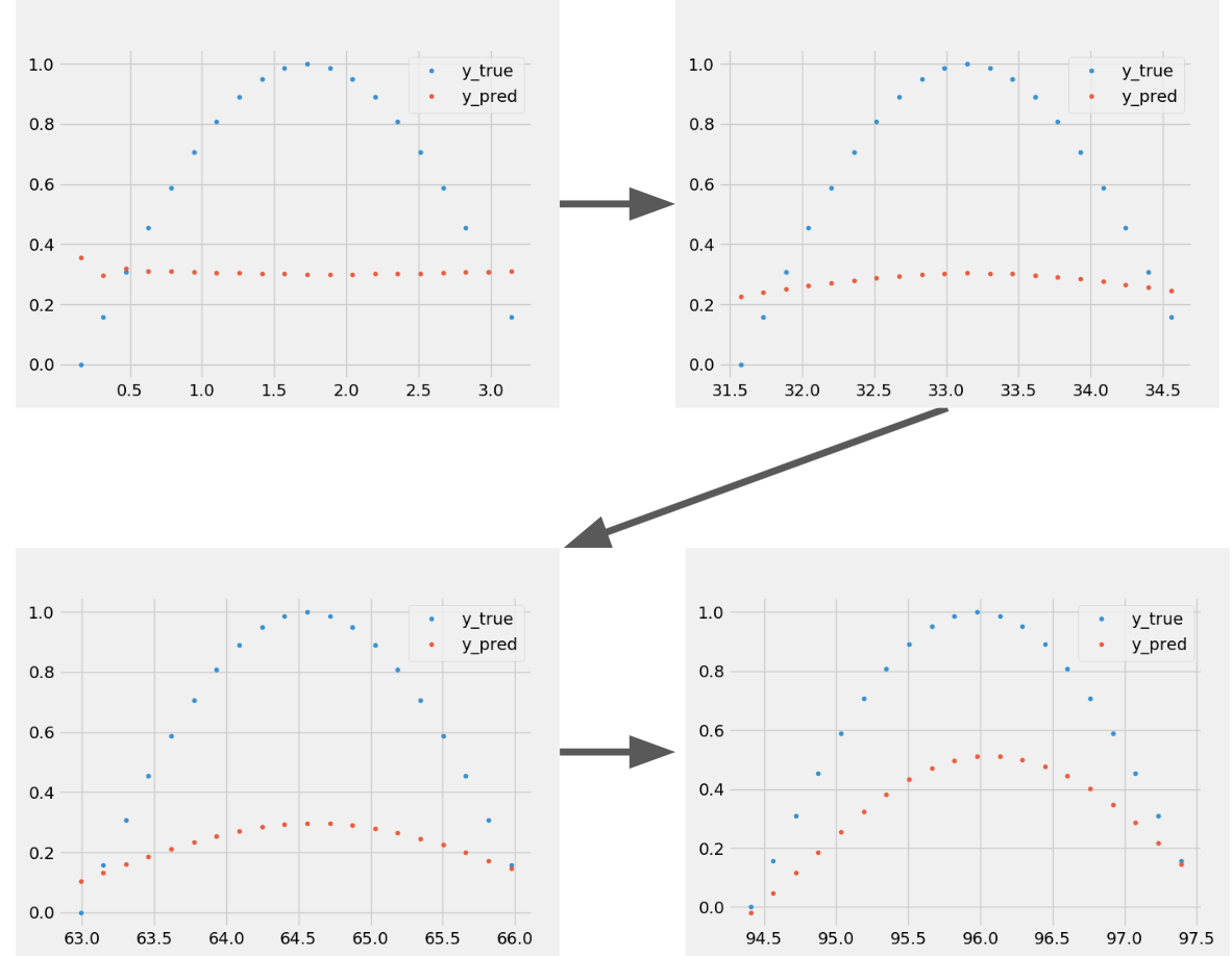
We can see that the model is slowly learning the function between X and Y.
But more importantly let's inspect what was printed out from the first few steps using much smaller values. By setting seq_len=1 we can "see" what's going on at every time step.
# decide on hyperparameters
input_size = 1  # 1 feature
output_size = 1  # 1 output
hidden_dim = 5  # let's keep this small for ease of inspection
n_layers = 1

# instantiate RNN
rnn = SimpleRNN(input_size, output_size, hidden_dim, n_layers)
print(rnn)
# simple MSE loss and Adam optimizer with a learning rate of 0.01
criterion = nn.MSELoss()
optimizer = torch.optim.Adam(rnn.parameters(), lr=0.01)

# train the rnn and monitor results
trained_rnn = train(rnn, criterion, optimizer,
                    seq_len=1, n_steps=3, print_every=10)
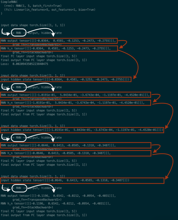
Red arrows represent data that is simply being passed forward while white arrows represent data that is undergoing some computation. The same RNN object performs the computation at each time step. We can see from this that the RNN behaves just like a simple recursive function; the input of the next step is the output from the previous!
- The output from the hidden layer for each data point is used as part of the input for the computation in the following time step.
- The output of the RNN is of the shape
(seq_len, hidden_dim), meaning that the output is simply the collection of outputs from the hidden layer for each time step (i.e. data point). The first row is the hidden layer output for the first data point in the sequence, so and so forth. To get the final output prediction for the entire sequence we flatten this and pass it through a finaly layer so that there is a prediction for each timestep (from the hidden output). - The output hidden tensor of the RNN is the final hidden layer output from the last time step (i.e. the last data point of the sequence).
- The output hidden tensor is also passed forward from batch to batch.